Introduction

SOLNP

The SOLNP algorithm by Yinyu Ye (1989) solves the general nonlinear optimization problem below. In other words, it will find an optimum (possibly local) to it. The algorithm was originally implemented in Matlab, and have gained some fame through it’s R implementation (RSOLNP). solnp is written in C++ and with the Python wrappers (pysolnp) you have seamless integration with Python, providing high efficiency and ease of use.

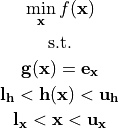
$\begin{gather*} \min_{\mathbf{x}} f(\mathbf{x}) \\ \textrm{s.t.} \\ \mathbf{g}(\mathbf{x}) = \mathbf{e}_\mathbf{x} \\ \mathbf{l}_\mathbf{h} < \mathbf{h}(\mathbf{x}) < \mathbf{u}_\mathbf{h} \\ \mathbf{l}_\mathbf{x} < \mathbf{x} < \mathbf{u}_\mathbf{x} \\ \end{gather*}$

Here:

$\mathbf{x}$ is the optimization parameter.
$f(\mathbf{x})$ , $\mathbf{h}(\mathbf{x})$ and $\mathbf{g}(\mathbf{x})$ are smooth constraint functions.
The constant-valued vector $\mathbf{e}_\mathbf{x}$ is the target value for the equality constraint(s).
The constant-valued vectors $\mathbf{l}_\mathbf{h}$ and $\mathbf{u}_\mathbf{h}$ are the lower and upper limits resp. for the inequality constraint(s).
The constant-valued vectors $\mathbf{l}_\mathbf{x}$ and $\mathbf{u}_\mathbf{x}$ are the lower and upper limits resp. for the parameter constraint(s).

Bold characters indicate the variable or function can be vector-valued. All constraints are optional and vectors can be of any dimension.

GOSOLNP

GOSOLNP tries to find the global optimum for the given problem above. This algorithm was originally implemented in R through RSOLNP, but has been made available in Python through the library pygosolnp.

This is done by:

Generate n random starting parameters based on some specified distribution.
Evaluate the starting parameters based on one of two evaluation functions (lower value is better):
1. Objective function $f(\mathbf{x})$ for all $\mathbf{x}$ that satisfies the inequality constraints $\mathbf{l}_\mathbf{x} < \mathbf{x} < \mathbf{u}_\mathbf{x}$
2. Penalty Barrier function: $f(\mathbf{x}) + 100 \sum_i(\max(0, 0.9 + l_{x_i} - [\mathbf{g}(\mathbf{x})]_i)^2 + \max(0, 0.9 + [\mathbf{g}(\mathbf{x})]_i - u_{x_i})^2) + \sum_j([h(\mathbf{x})]_j - e_{x_j})^2/100$
For the m starting parameters with the lowest evaluation function value, run pysolnp to find nearest optimum.
Return the best converged solution among the ones found through the various starting parameters (lowest solution value.)